# @title Fusion Impact on the Roofline { display-mode: "form" }
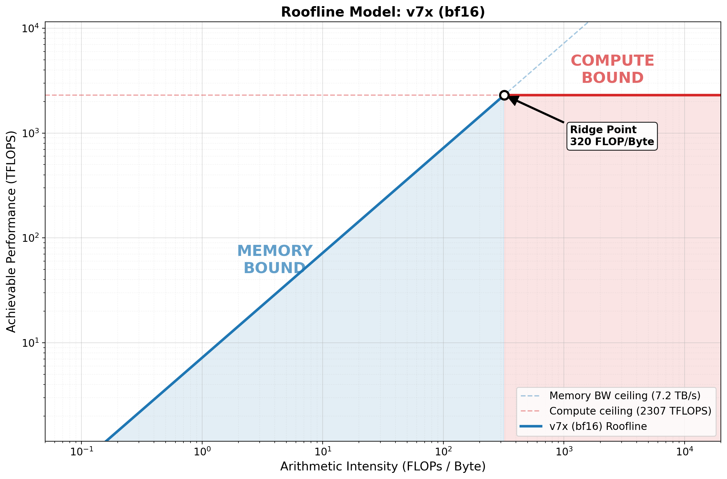
hw = HW_SPECS["v7x (bf16)"]
ai_vals = np.logspace(np.log10(0.05), np.log10(20000), 500)
roofline_vals = np.minimum(ai_vals * hw['peak_bw'], hw['peak_flops'])
fig, ax = plt.subplots(figsize=(12, 8))
# Draw roofline with colored segments
ridge = hw['ridge']
mask_mem = ai_vals <= ridge
mask_comp = ai_vals >= ridge
ax.loglog(ai_vals[mask_mem], roofline_vals[mask_mem], '-', color='#1f77b4', linewidth=3)
ax.loglog(ai_vals[mask_comp], roofline_vals[mask_comp], '-', color='#d62728', linewidth=3,
label=f'v7x (bf16) Roofline')
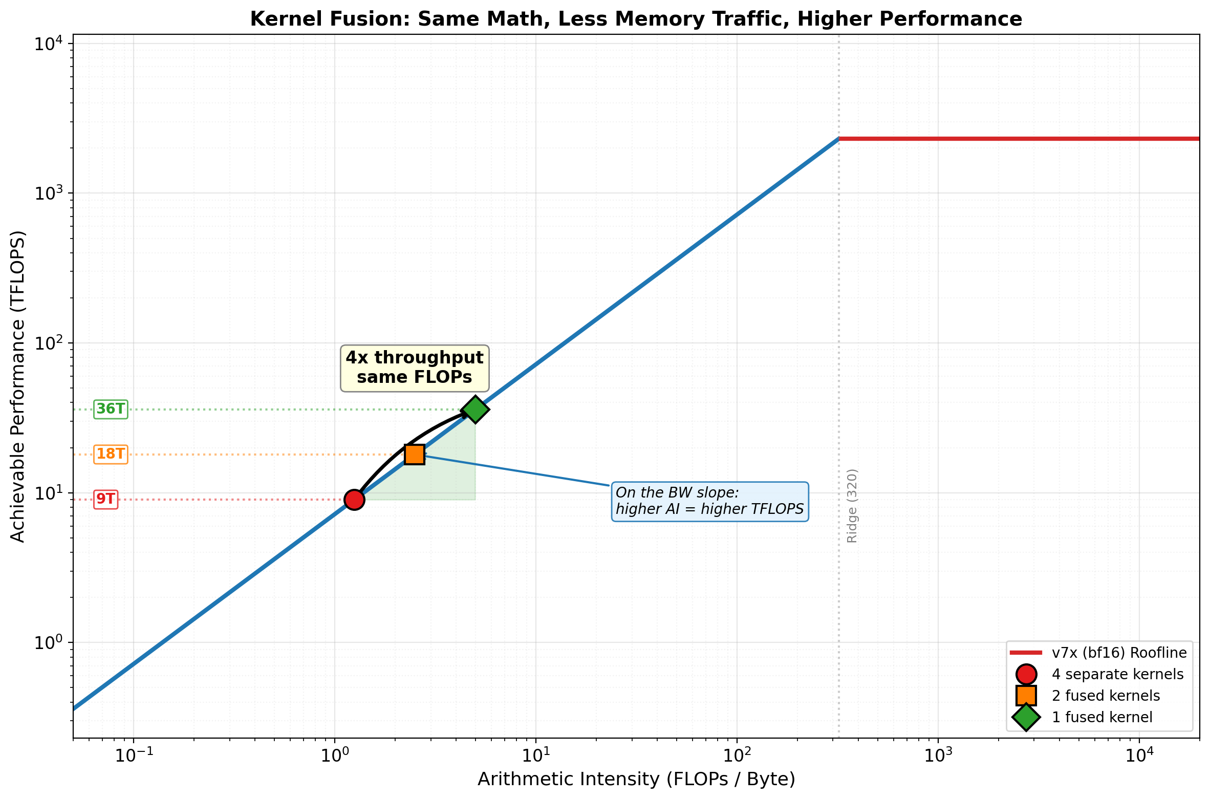
# --- Scenario: A transformer block's elementwise tail ---
# Unfused: LayerNorm -> GELU -> Dropout -> Residual Add (4 separate kernels)
# Each reads from HBM and writes back to HBM
num_el = 32 * 2048 * 4096 # batch * seq * hidden
dtype = 2 # bf16
one_rw = 2 * num_el * dtype # one read + write round trip in bytes
# Unfused: 4 separate kernels, each does a read+write round trip
unfused_flops = num_el * (10 + 8 + 1 + 1) # LN(10) + GELU(8) + Dropout(1) + Add(1)
unfused_bytes = 4 * one_rw # 4 kernels, each reads + writes
unfused_ai = unfused_flops / unfused_bytes
# 2-way fused: (LayerNorm+GELU) and (Dropout+Add) — 2 kernels
fused2_flops = unfused_flops
fused2_bytes = 2 * one_rw
fused2_ai = fused2_flops / fused2_bytes
# Fully fused: all 4 ops in one kernel — 1 read, 1 write
fused4_flops = unfused_flops
fused4_bytes = one_rw
fused4_ai = fused4_flops / fused4_bytes
# Compute roofline performance for each
scenarios = [
("4 separate\nkernels", unfused_ai, unfused_bytes, '#e41a1c', 'o', 14),
("2 fused\nkernels", fused2_ai, fused2_bytes, '#ff7f00', 's', 14),
("1 fused\nkernel", fused4_ai, fused4_bytes, '#2ca02c', 'D', 14),
]
unfused_perf = roofline_perf(unfused_ai, hw['peak_flops'], hw['peak_bw'])
fused4_perf = roofline_perf(fused4_ai, hw['peak_flops'], hw['peak_bw'])
# Shade the performance gain region between unfused and fused on the roofline
shade_mask = (ai_vals >= unfused_ai) & (ai_vals <= fused4_ai)
ax.fill_between(ai_vals[shade_mask], unfused_perf, roofline_vals[shade_mask],
color='#2ca02c', alpha=0.15)
# Plot each scenario as a dot on the roofline
for label, ai, nbytes, color, marker, ms in scenarios:
perf = roofline_perf(ai, hw['peak_flops'], hw['peak_bw'])
# Dot on the roofline
ax.plot(ai, perf, marker, color=color, markersize=ms,
markeredgecolor='black', markeredgewidth=1.5, zorder=5, label=label.replace('\n', ' '))
# Horizontal dashed line to y-axis showing the TFLOPS value
ax.plot([ai_vals[0], ai], [perf, perf], ':', color=color, alpha=0.5, linewidth=1.5)
# TFLOPS label on the y-axis side
ax.text(ai_vals[0] * 1.3, perf, f'{perf:.0f}T', fontsize=10, fontweight='bold',
color=color, va='center', ha='left',
bbox=dict(boxstyle='round,pad=0.15', fc='white', ec=color, alpha=0.8))
# Big arrow from unfused to fused with "4x" annotation
ax.annotate('', xy=(fused4_ai, fused4_perf), xytext=(unfused_ai, unfused_perf),
arrowprops=dict(arrowstyle='->', color='black', lw=2.5,
connectionstyle='arc3,rad=-0.15'))
mid_ai = 10**((np.log10(unfused_ai) + np.log10(fused4_ai)) / 2)
mid_perf = 10**((np.log10(unfused_perf) + np.log10(fused4_perf)) / 2)
ax.text(mid_ai, mid_perf * 3, f'4x throughput\nsame FLOPs',
fontsize=12, ha='center', fontweight='bold',
bbox=dict(boxstyle='round,pad=0.3', fc='lightyellow', ec='gray', alpha=0.95))
# Key insight annotation: why moving right = moving up on BW slope
ax.annotate('On the BW slope:\nhigher AI = higher TFLOPS',
xy=(fused2_ai, roofline_perf(fused2_ai, hw['peak_flops'], hw['peak_bw'])),
xytext=(fused4_ai * 5, unfused_perf * 0.8),
fontsize=10, ha='left', style='italic',
arrowprops=dict(arrowstyle='->', color='#1f77b4', lw=1.5),
bbox=dict(boxstyle='round,pad=0.3', fc='#e3f2fd', ec='#1f77b4', alpha=0.9))
# Ridge line annotation
ax.axvline(x=ridge, color='gray', linestyle=':', alpha=0.4)
ax.text(ridge * 1.1, hw['peak_flops'] * 0.002, f'Ridge ({ridge:.0f})',
fontsize=9, color='gray', rotation=90, va='bottom')
ax.set_xlabel('Arithmetic Intensity (FLOPs / Byte)', fontsize=13)
ax.set_ylabel('Achievable Performance (TFLOPS)', fontsize=13)
ax.set_title('Kernel Fusion: Same Math, Less Memory Traffic, Higher Performance',
fontsize=14, fontweight='bold')
ax.legend(fontsize=10, loc='lower right')
ax.set_xlim(0.05, 20000)
ax.set_ylim(hw['peak_flops'] * 0.0001, hw['peak_flops'] * 5)
ax.grid(True, which="major", alpha=0.3)
ax.grid(True, which="minor", alpha=0.15, linestyle=':')
plt.tight_layout()
plt.show()
# Summary table
print("Scenario: LayerNorm -> GELU -> Dropout -> Residual Add")
print(f" Elements: {num_el:,} (batch=32, seq=2048, hidden=4096)\n")
print(f" {'Strategy':<22} | {'HBM Traffic':>12} | {'AI':>8} | {'Roofline Perf':>14} | {'Speedup':>8}")
print(f" {'-'*76}")
for label, ai, nbytes, _, _, _ in scenarios:
name = label.replace('\n', ' ')
perf = roofline_perf(ai, hw['peak_flops'], hw['peak_bw'])
speedup = perf / unfused_perf
traffic_gb = nbytes / 1e9
print(f" {name:<22} | {traffic_gb:>9.2f} GB | {ai:>8.1f} | {perf:>10.1f} TFLOPS | {speedup:>7.1f}x")
print(f"\n All three are memory-bound — but that's the point. On the BW slope,")
print(f" every 2x reduction in memory traffic is a 2x improvement in throughput.")
print(f" Fusion doesn't change the FLOPs — it eliminates redundant HBM round-trips.")